We thank Madhusudhan B A, Ara Ramalingam and Muthupandian Thangarajan for their guidance and support towards making this paper a reality
Abstract
We implemented the SegNet neural network architecture to detect strays of transparent and colored plastic on a conveyor belt containing paper from recycled garbage at a recycling / sorting facility in California and to determine whether this architecture was suitable for single object detection. We have also analyzed the performance of the model generated during the different stages of training on our test set to identify patterns if any.
SegNet was designed to be an efficient architecture for pixel-wise semantic segmentation and it was our opinion that a pixel-wise semantic segmentation will aide in detecting the contours of plastic. FCN1 is also a popular architecture for pixel-wise segmentation but we chose SegNet as the authors of SegNet claim that their architecture was more efficient in terms of memory, accuracy, computation time compared to FCN and also used fewer trainable parameters.
An alternate was to try the faster R-CNN2. Since one of our initial requirements was to identify contours of the plastic, we did not consider Faster R-CNN as it would have only provided us with bounding boxes.
1.Introduction
 Our aim was to do identify strays of transparent plastic on a moving conveyor belt containing mostly paper at a garbage sorting facility using SegNet and to determine if it is the right method to solve our problem.
SegNet is a deep fully convolutional neural network for pixel-wise segmentation.
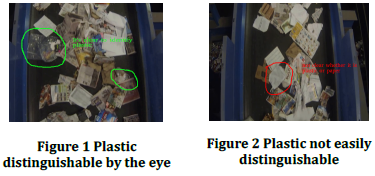
The main challenge we faced was that, even visually, it was not possible to identify plastic in certain cases.
Figure 1 and 2 serves as an example. Figure 1 can be clearly concluded as plastic while in Figure 2 it is unclear.
2.Architecture
This SegNet architecture was derived from the deep FCN. 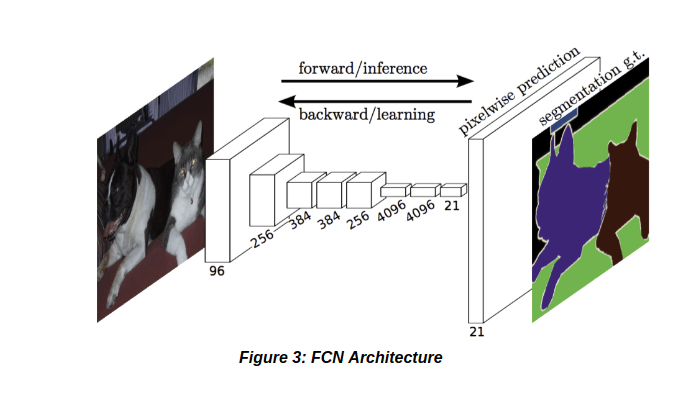 It consists of two parts – an encoder and a decoder. The encoder is similar to the VGG163, but without the fully connected layer thus making the model smaller. The decoder consists of the deconvolutional network which is used for the upsampling process. This upsampling is done for accurate pixel-wise classication and to increase the resolution of the downsampled feature maps. Every decoder has a corresponding encoder.
The decoder makes use of the max-pooling indices which is obtained from the corresponding encoder to perform upsampling of the feature maps from the encoder. 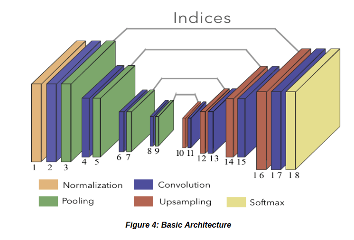 The reusing of max-pooling indices helps in reducing the training parameters and also improves the boundary delineation.
We have made use of the SegNet – Basic architecture. This consists of four convolutional layers in encoder coupled with batch normalization and ReLu followed by a maxpooling layer.
Decoder consists of the same but instead of the max-pooling layer an upsampling layer is present. The architecture of FCN and SegNet-Basic have been shown in Figure 3 and Figure 4 respectively.
3.Dataset preparation
Step 1: Dataset Collection & Preparation
Our source data was a video shot through an entry level mobile phone camera. We collected the images by cutting frames from the video. The images were resized as our model takes an input of 480px of width and 360px of height. Then we took a total of 1,000 images such that 750 images contained plastic and 250 images were just paper without any plastic. Allotted a total of 600 images of plastic and 150 images without plastic to the training set and the rest to the validation set.
Step 2: Dataset Ground Truth
We annotated the dataset using SegNet-annotate-tool4 . The annotation tool produces an output in a format which is not readily acceptable by the SegNet algorithm. We were able to suitably handengineer and automate the conversion process so that the output format was acceptable.
Step 3: Weight Calculation
The weights5 have to be calculated using the train set. These weights are used to calculate the loss during the training process. According to the SegNet paper, when there is a large variation in the number of pixels in each class in the training set there is a requirement to weight the loss differently. This is known as class balancing.
4.Training the model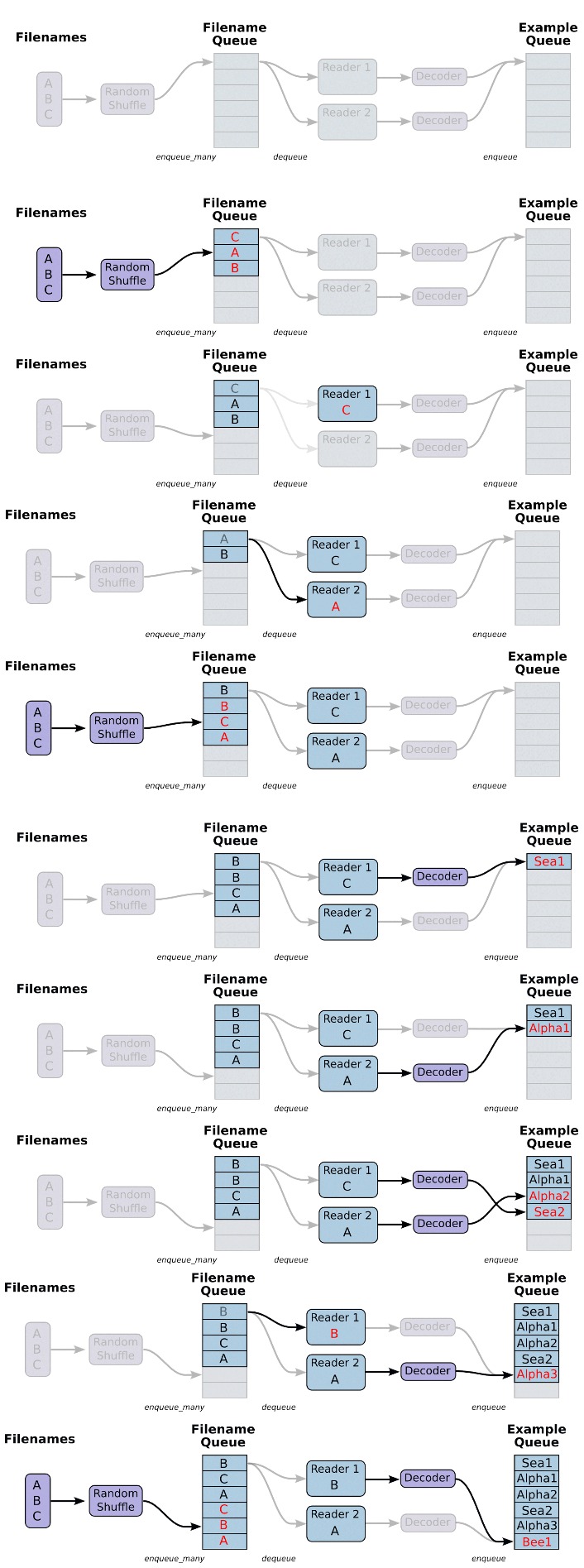
The process of training involves passing batches of the train images to the network using a concept of input pipeline. This input pipeline involves the use of two main queues, filename queue and example queue. Filename queue collects the filenames, which are passed through a decoder and enqueued to the example queue where the images are dequeued and passed to the network in batches and the training process starts. Figure 5 illustrates this process, this process is called input pipelining.
We used an input of 360 x 480 on an NVIDIA GeForce GTX 1050Ti with cuDNN6 v6 acceleration. There are two variants of the SegNet architecture – first the standard SegNet and second the SegNet Basic.
The rst variant being standard SegNet architecture makes use of 13 convolutional layers in both encoder and decoder networks. We tried this on our 4GB GTX 1050Ti GPU, but, encountered a CUDA7 out of memory error.
Since all the images which we pass to the network in batches are stored in the GPU memory, the more layers we use the more memory gets utilized and thus we encountered this CUDA out of memory error. Then we tried reducing the layersby half to six layers and still encountered the same problem. Then we tried the second variant SegNet – Basic which makes use of four convolutional layers in both encoder and decoder networks as shown in Figure 4. This ran smoothly on our GPU and thus we made use of the egNet-Basic architecture. Figure 5 Input Pipeline to pass images to the network
At each step of the training process the mean Intersection over Union (mIoU), loss and accuracy is calculated for the the batch of training set.
4.1.The mIoU is calculated by using the following formula :

Where : True Positive[TP] is the number of pixels correctly classified as positive, False Positive[FP] is the number of pixels wrongly classified as positive, False Negative[FN] is the number of pixels wrongly classified as negative
4.2.The accuracy value is calculated using the following formula:

Where: True Negative [TN] is the number of pixels [n(px)] correctly classified as negative. The loss is calculated by using the the ground truth image as well as the SegNet networks output using the pixel values (These images are gray images). At every 100 steps the mean Intersection over Union, loss and accuracy is calculated for the validation set. The graphs for the above process is maintained in a TensorBoard8 and the values are maintained in a csv. At every 1,000 steps the models checkpoint file (which consists of model weights to test our model) will be saved.
5.Hyper-parameter settings
We first set the maximum steps to 30,000. The validation loss started increasing approximately from the 6,000th step but when it reached the 15,000th step it started increasing at a faster rate thus we chose the maximum steps to be 15,000. Batch size is the number of images passed to the network at every step of the training process. The higher the batch size the more sooner the training would complete. We chose three values for our batch size and they are as follows:
5.1.Training with batch size 6
Batch-size = 6, Learning rate = 0.001, min-after-dequeue9 = 0.4 X (Size of training set), max-steps = 15,000 When we used batch size of 6 we encountered the CUDA out of memory error which we have mentioned about earlier.
5.2.Training with batch size 5
Batch-size = 5,
Learning rate = 0.001,
min-after-dequeue = 0.4 X (Size of training set), max-steps = 15,000
This ran smoothly without any errors.
5.3.Training with batch size 4
Batch-size = 4,
Learning rate = 0.001,
min-after-dequeue = 0.4 X (Size of training set), max-steps = 15000
We tried the same using batch size 4 to check if this hyperparameter(batch-size) has a significant impact on the performance and accuracy. Repeated the training five times for both batch size 4 and batch size 5.
5.4.Steps and epochs
At every step, x number of images are passed to the network where x is the batch size. Thus one epoch is completed once all the images in our training set have been passed on to the network.

Where ts is the training set and bs is the batch size.
Example: Since we have used a batch size of 4, 1 epoch will be completed in approximately 188 steps. In that case 15000 steps would correspond to almost 80 epochs.
6.Analysis of the training process
The TensorBoard results for validation accuracy and validation loss for both the batch sizes are shown below.
6.1.Batch Size 4
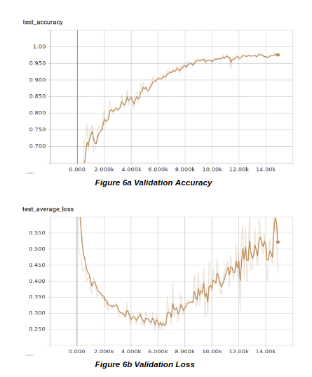
The validation loss in the case of batch 4 reached a minimum of 0.2450 at the 5,800th step and from there on it started increasing. The figures 6a and 6b illustrate this.
6.2.Batch Size 5
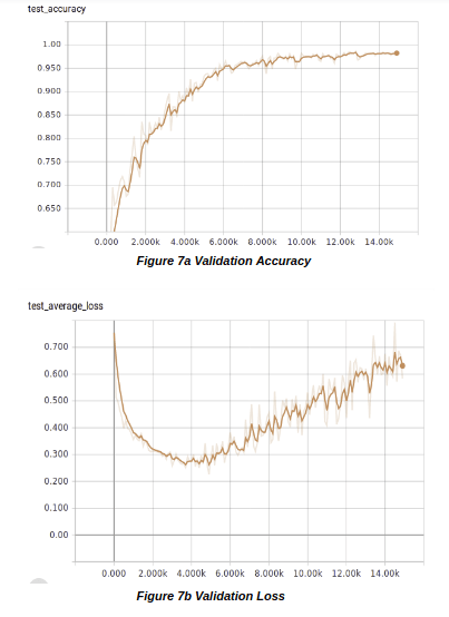 The same kind of behaviour was observed in the case of batch 5, only difference was that the increase in loss started at the 4,900th step with a loss of 0.2258 which is shown in Figure 7a and 7b. The training loss in both the cases of batch size were gradually decreasing. But there was a sudden increase in the validation loss while the training loss continued to decrease from which we concluded that the model was overfitting.
Next we created a test set of 150 images with 101 of them having plastic and 49 without plastic. We used every checkpoint of the model to test on our test set. The reason for using all the checkpoints was to analyze the differences in the model’s result at different steps. Since we maintained a checkpoint le every 1,000 steps we had a total of 15 checkpoints. We found that the batch size 5 model performed slightly better than batch size 4 model.
7. Results from the model
7.1.Pass Cases
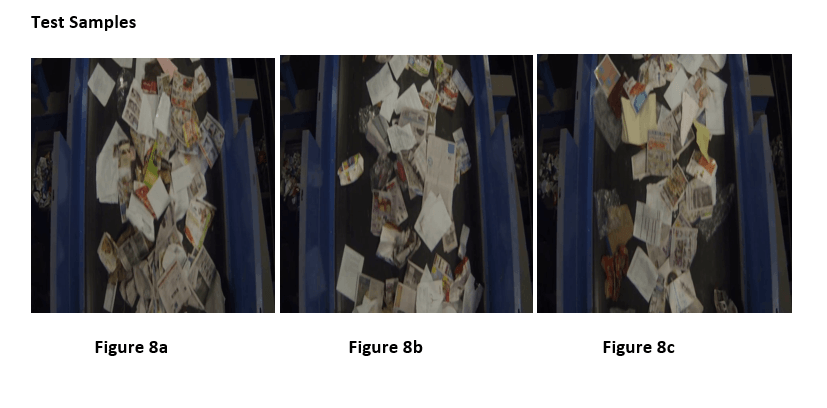
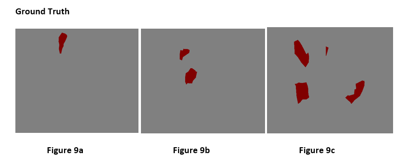
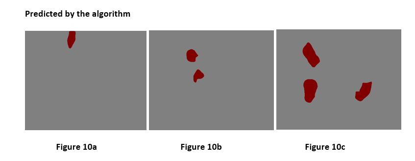
7.2.Failed Cases
The results were not perfect and to analyze the results we created our own set of categories to classify the results to compare the performance between different checkpoint files. We first tried to obtain a single number metric to categorize the results but this was not possible as the predicted results were not confined to a fixed number of cases. Example: Some cases involved the predicted plastic to be correctly located but the size of the blob varied from the ground truth. Another case where the plastic was detected correctly but extra non existent plastics were also detected along with it.
To overcome this, we came up with a total of 6 unique categories for the images with plastic as shown Table 1. Our test set contained 101 images with plastic and 49 without plastic. We maintained a separate table for both.
The main reason we considered the columns B (Table 1) as true positive is because our aim was to make sure the model detects all plastic regardless of the paper detected along with it. If our aim were to detect plastic without detecting a single paper we would have to consider the columns B (Table 1) as False Negative. The images without plastic have two categories either True Negative or False Positive as shown in Table 2. Table 1 gives a brief explanation of each category, for Table 2 the True Negative are those cases where there is no plastic in the image and the model also predicted the same, whereas False Positive are those cases where there is no plastic 6 in image but the model has predicted some non existent plastic.
7.3.An excerpt of the sheet we maintained:
The categories which are significant in defining the performance of our model are in columns A (Table 1)
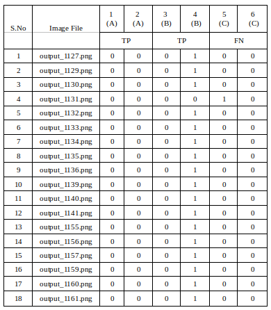
1 – Location of the detected plastics and size of it are perfect matched with the visual appearance
2 – Locations are precise, but difference in the size of the plastics
3 – Plastic locations and size are correct, but predicted plastics at additional locations.
4 – Plastic locations precise with different sizes, also predicted plastics at additional locations
5 – Not detected any plastics but showing ones where it doesn’t exist
6 – No plastic detected
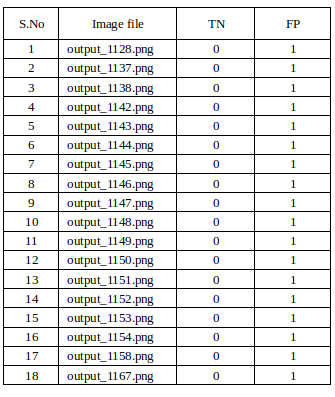
A common pattern that we observed during our analysis of test set on different checkpoint files (for both batch size 4 and 5) was that the number of extra non-existent plastic decreased whereas the number of null predictions increased as the steps increased.
8.Increasing the Size of the Dataset
We found that a common reason for overfitting is usually due to a small dataset where the model usually tends to memorize the training images along with its corresponding labels and the model settings would be very specific to the train set. Then we increased the dataset from 1000 images to 2000 images of which we allotted 1500 images to train set and the rest to validation set. The graph of validation loss was no different (gradual decrease with a sudden increase) expect for the fact that the validation loss reduced, and the increased datasets model performed much better and got more True positives compared to the one we trained with 750 image.
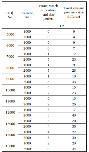
From the above Table 3 it is clear that, the number of True Positives (TP) are higher at every stage for the 2,000 images dataset. And then, we made use of the same 2,000 images and considered 1,750 images as the training set and 250 images as the validation set. The result of this training gave a significant decrease in the loss to 0.1848 at the 9,300th step and started increasing from there on. Thus from the above results, we concluded the size of the dataset has a significant impact on the accuracy and validation loss value.
9.Dropout inclusion
 The most efficient way to avoid the problem of overfitting is to include a dropout layer, but, when we ran the code with the included dropout on our NVIDIA GeForce GTX 1050 Ti, we once again encountered the CUDA out of memory error.
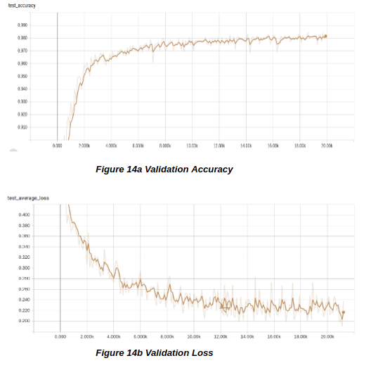
To solve this problem, we ran the same code on Google Colab10 on a 12GB GPU with the 2,000 images dataset and the result of the validation loss graph showed no sudden increase as in the previous runs. The dropout layer significantly reduced the problem of overfitting but the loss value did not go below 0.1840. The graphs have been shown below in Figure 14a and 14b.
10.Challenges
It was very dificult to segregate the images with plastic and without plastic visually. We found it dificult to find a single valued metric for classifying the test results but came up with a fixed set of categories to categorize them as explained earlier.
11.Additional process with different dataset
 We did not get the required accuracy for the plastic dataset. We assumed that the dataset might have been too small for such a complex network like SegNet which involves the use of lot of parameters. To check, if this holds true we took a smaller dataset of 1,000 images of T-shirts compared to our 2,000 images of plastic.
We had an idea to make the process of purchasing shirts more engaging and interactive by which users could select the t-shirt they like on a screen and this would be correctly placed on the body of the user, which can be viewed on the same screen below. To accomplish this task, we required the Tshirt which a person was wearing, to be correctly segmented out. SegNet was the perfect architecture as it was capable of delineating the boundaries by which the exact shape of the shirt could be extracted. For this we downloaded images of people wearing t-shirts from the internet. We took this new dataset to see, if the image quality also had a significant impact on the detection results.
 We took a total of 1,045 images allotted 900 as the training set and the rest as the validation set. We used an input of 360 X 480 on an NVIDIA GeForce GTX 1050Ti with cuDNN v6 acceleration. The labeling of these images were easy for us compared to the plastic labeling.
The images were of high quality compared to the plastic dataset which was mediocre.
We trained the model with the following hyperparameters:
Batch-size=5,
Learning rate=0.001,
min-after-dequeue= 0.4 x (Size of training set), max-steps= 20000
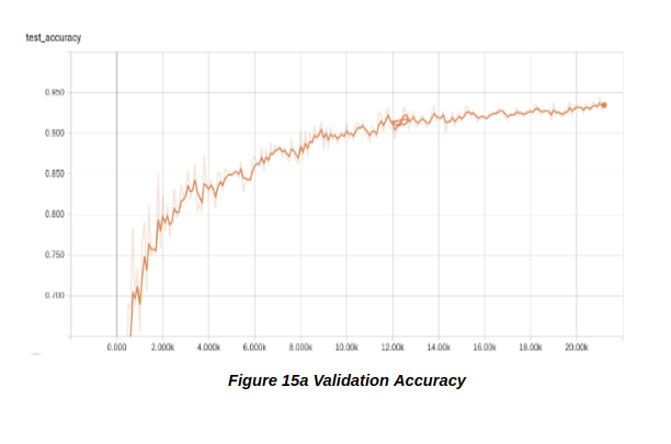
Once the training of the t-shirts completed, we observed that there was a gradual decrease without any sudden increase in the validation loss value. The curve that we were expecting from our plastic dataset. The validation loss reached a minimum of 0.05 which was significantly better (Figure 15a & 15b).
12.Sample results of the t-shirt dataset
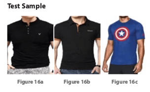
We succeeded in segmenting out the t-shirts a person is wearing, which is clear from the above results. From this additional process, we learnt that a small dataset was sufficient to obtain a good accuracy with minimal loss. We also found that increasing the dataset may not have a significant impact on accuracy and loss as proved by the plastic dataset, unless the image quality is good. Thus we identified that the required result could be achieved using a small dataset provided that we have a clear or unambiguous dataset.
From this we could conclude that the dataset size is not a limiting factor for accuracy and the quality of images do play a vital role in obtaining a good accuracy.
13.Quantitative comparison


